INTRODUCTION
There have been many requests for improvements to the Dropdown list from Smartsheet Community.
The two most typical requests are
- Automatic updating of the list
- Dynamically changing the list of the following selections based on previous selections
Regarding the first, automatic updating of the list, users want a master sheet of dropdown lists, so changing the list will change the options on the target sheet’s dropdown lists. Since this functionality is unavailable, the user must manually update the list.
As for the second, dynamically changing the list of the following selections based on previous selections, some mimic dynamic or dependent dropdown lists, using form logic to display a specific column of choices based on the previous selections, preparing columns for the options in advance. However, this method also requires manual preparation of the columns of choices and works only for the form.
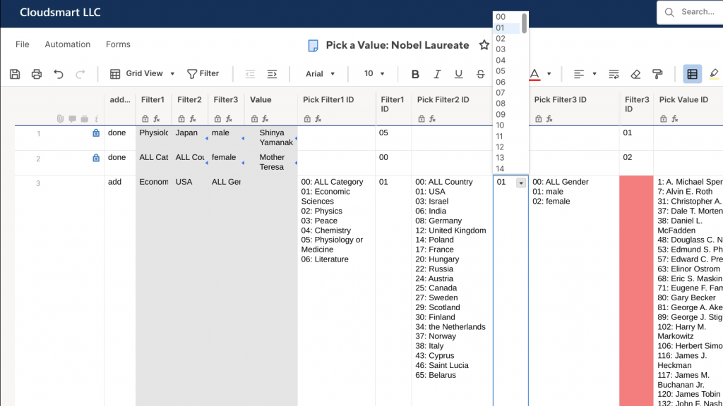
To solve this problem, we have devised a workaround that displays a list of two-digit numeric IDs and dropdown list items in a cell so that users can enter the two-digit numeric IDs corresponding to a list item.
Although it is not as easy as a dropdown list, where you can click on a choice and the selection is complete, our method requires you to enter a two-digit number, so it is not much of a hassle. You can prepare the two-digit number choices and have the user click on them.
For more information, please refer to the sample dashboard in the following link.
https://app.smartsheet.com/b/publish?EQBCT=2580af6de6e845758f74b6556396d9ee
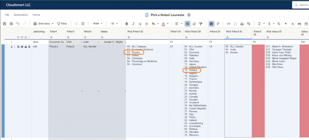
To illustrate the use of the method, let’s take the example of selecting Nobel laureates. In this example, you choose a category such as Physics or Chemistry as the first filter, then a list of countries is displayed as the second filter based on the first filter. And, if you select a specific country, a third filter is shown with a gender. Then when you choose a particular gender, a formula displays a list of candidates.
All of these lists are in the form of a ‘two-digit ID: choice.’
How it works
Composition of the sheet
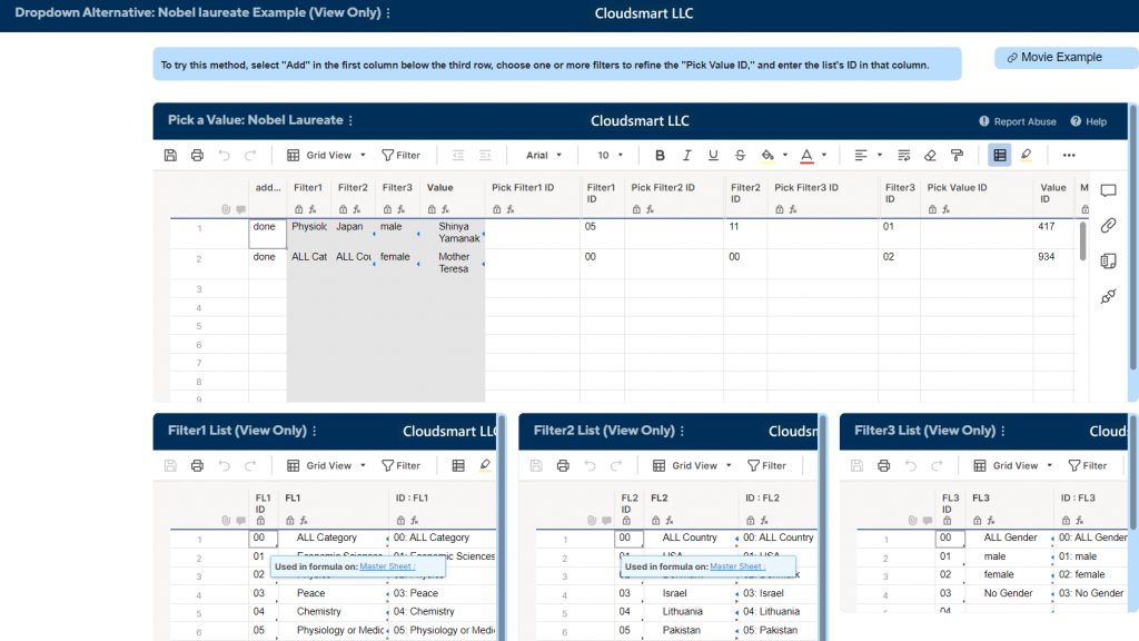
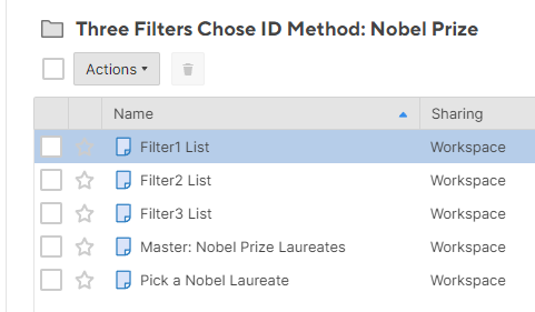
In this method, we use the following three types of sheets. (A demo three-filter example consists of five sheets.)
- Master sheet
- ID creation sheets (Filter1 List, Filter2 List, Filter3 List, if you use three criteria or filters to select a value)
- Pick a Value sheet
A mechanism for automatic updating of the list
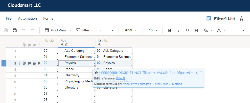
(At the ID creation sheet, Filter 1 List, for example)
The “ID creation sheets” create a list of unique values from the master sheet and pairs the list with two-digit numbers.
- Column 1.
- The first column, [FL1 ID], is pre-populated with 00 to 99.
- Example: 02
- Column 2.
- =IFERROR(INDEX(DISTINCT({FLT1}), VALUE([FL1 ID]@row) + 1), “”)
- Example: Physics
- Column 3.
- =IF(ISTEXT([FL1]@row), [FL1 ID]@row + “: ” + [FL1]@row, “”)
- Example: 02: Physics
Where {FLT1} is the Filter1: first filter (or category) column on the master sheet.
For example, suppose that the column {FLT1} has the following data.
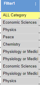
The above formula produces the following tabular table.
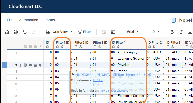
In the master sheet, the following formula will calculate, based on the table above, the values in the [ID: FL1] column (e.g., 02: Physics) corresponding to the respective data (e.g., Physics).
- =INDEX({FL1 ID}, MATCH([FIlter1]@row, {FL1}, 0))
- =[FIlter1 ID]@row + ” : ” + [FIlter1]@row
How the Pick a Value sheet displays the first list
The Pick a Values sheet has the following fields in Sheet Summary that a formula like this creates;
- =JOIN({ID : FL1}, CHAR(10))
fl.1
- 00: ALL Category
- 01: Economic Sciences
- …
fl.2
- 00: ALL Country
- 01: USA
- …
fl.3
- 00: ALL Gender
- 01: male
- …
To show the list only when necessary, the Pick a Value sheet has a column, [add/chng], with a dropdown list with {“Add,” “Change,” and “Done”} options.
When a user selects “add” or “change,” the sheet displays the first list with the following formula;
- =IF(OR([add/chng]@row = “Add”, [add/chng]@row = “Change”), [fl.1]#, “”)
(Note: When the user finishes “Add” or “Change” by inputting the value ID, the workflow automation changes the value of [add/chng] to “Done” to hide the lists.
How the Dynamic Dropdown or Dependent Dropdown List works
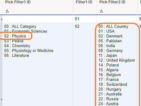
When the user enters the first 2-digit ID, the candidate column for the second filter (category) displays a list based on the first selection with the following formula.
- =IF(VALUE([Filter1 ID]@row) = 0, [fl.2]#, INDEX({ID : FL2 of ALL List}, 1) + CHAR(10) + JOIN(DISTINCT(COLLECT({ID : FL2 of ALL List}, {FL1 ID of All List}, VALUE(@cell) = VALUE([Filter1 ID]@row))), CHAR(10)))
The functionality of a Dynamic (or Dependent) Dropdown List
- =JOIN(DISTINCT(COLLECT({ID : FL2 of ALL List}, {FL1 ID of All List}, VALUE(@cell) = VALUE([Filter1 ID]@row))), CHAR(10))
Here, the {ID: FL2 of ALL List} is the range for the second ‘two-digit ID: choice’ column on the master sheet.
In plain English, the above formula means joining distinct values of the second ‘two-digit ID: choices’ of rows that have the same first filter ID as the user has chosen in the first step.
The first part of the formula assumes the user selects “ALL.”
- =IF(VALUE([Filter1 ID]@row) = 0, [fl.2]#, INDEX({ID : FL2 of ALL List}, 1) + CHAR(10) + JOIN(DISTINCT(COLLECT({ID : FL2 of ALL List}, {FL1 ID of All List}, VALUE(@cell) = VALUE([Filter1 ID]@row))), CHAR(10)))
If the user selects “All: 00” in the previous step, the formula display all Filter 2 options.
The primary mechanism is as described above, and the column that displays the final candidate values is a relatively complex expression of 1208 characters, excluding spaces so that if a user selects ALL in any one or two filters in the three filter columns, the corresponding value and its ID pair is also displayed.
- =IF(AND(VALUE([Filter2 ID]@row) = 0, VALUE([Filter3 ID]@row) = 0), JOIN(COLLECT({ID : Value of All List}, {FL1 ID of All List}, VALUE(@cell) = VALUE([Filter1 ID]@row)), CHAR(10)), IF(AND(VALUE([Filter1 ID]@row) = 0, VALUE([Filter3 ID]@row) = 0), JOIN(COLLECT({ID : Value of All List}, {FL2 ID of All List}, VALUE(@cell) = VALUE([Filter2 ID]@row)), CHAR(10)), IF(AND(VALUE([Filter1 ID]@row) = 0, VALUE([Filter2 ID]@row) = 0), JOIN(COLLECT({ID : Value of All List}, {FL3 ID of All List}, VALUE(@cell) = VALUE([Filter3 ID]@row)), CHAR(10)), IF(VALUE([Filter1 ID]@row) = 0, JOIN(COLLECT({ID : Value of All List}, {FL2 ID of All List}, VALUE(@cell) = VALUE([Filter2 ID]@row), {FL3 ID of All List}, VALUE(@cell) = VALUE([Filter3 ID]@row)), CHAR(10)), IF(VALUE([Filter2 ID]@row) = 0, JOIN(COLLECT({ID : Value of All List}, {FL1 ID of All List}, VALUE(@cell) = VALUE([Filter1 ID]@row), {FL3 ID of All List}, VALUE(@cell) = VALUE([Filter3 ID]@row)), CHAR(10)), IF(VALUE([Filter3 ID]@row) = 0, JOIN(COLLECT({ID : Value of All List}, {FL1 ID of All List}, VALUE(@cell) = VALUE([Filter1 ID]@row), {FL2 ID of All List}, VALUE(@cell) = VALUE([Filter2 ID]@row)), CHAR(10)), JOIN(COLLECT({ID : Value of All List}, {FL1 ID of All List}, VALUE(@cell) = VALUE([Filter1 ID]@row), {FL2 ID of All List}, VALUE(@cell) = VALUE([Filter2 ID]@row), {FL3 ID of All List}, VALUE(@cell) = VALUE([Filter3 ID]@row)), CHAR(10))))))))
Usage
The usage of this method is as follows.
Demo Video
- Copy the above five sheets for each folder or workspace.
- Paste the data of Filter1, Filter2, Filter3, and the value structure into the master sheet.
- Delete unnecessary rows from the master sheet.
- Edit each filter column in the first row of the master sheet to show the filter name (category name) of what ALL is. (e.g., ALL → country ALL)
- Open the three ID creation sheets and update the references.
- Make sure the references updates are working in the master sheet, e.g., ID ID ID: FL1.
- You may need more IDs for your template if you use a dataset with several hundred rows. In such a case, go to the filter and master sheets and check for enough IDs.
- Pick up the values on the pickup sheet.
- Based on the picked-up values, edit the master sheet to reference related data.
- I got the dataset from Kaggle, etc., and have displayed the samples I created on my dashboard by doing steps 1-8 above for the Nobel Laureates, Cars, Movies, and Employee Directory cases.
Once you get used to it, the process takes about 15 minutes.
Summary
Regarding the following pains of the Smartsheet Dropdown list, we consider our solution practical enough to introduce to the Smartsheet community.
- Automatic updating of listings
- Dynamically changing the following listing based on the previous selection
FYI, this solution automatically generates the ID lists to save the user time and effort. Still, if you already have an ID, you can delete the formula in the column of the ID creation sheet (make it a cell formula) and look back to a unique ID.